The Nonlinear Optics Web Site

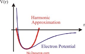
Dipole in a Static Electric Field

To understand nonlinear-optics, it is useful to first consider the case when the electric fields are time independent. Furthermore, we reduce the problem to one dimension where the fields and dipole moments point in the same direction. Thus, all quantities can be treated as scalars.

The figure below shows the potential energy of a charge in a material as a function of position, r, relative to some center of force. The sharp increase of the potential at the origin acts as a wall that keeps the charge from reaching the origin. The bottom of the well represents the equilibrium position of the charge.

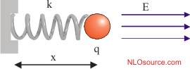
A particle attached to a spring can be represented by this type of potential. When the spring is fully compressed, it pushes against the wall. In the other extreme, for large enough extensions, the spring no longer obeys Hook's law, and the charge becomes free after the spring has unraveled and breaks.

The figure below show a charged particle attached to a spring. A force is applied to the charge through the electric field.

The most general model for the dipole moment, which is proportional to the extension of the spring, is a series of the electric field,

where p₀ is the dipole moment with no field applied, α is called the polarizability, β the hyperpolarizability, γ the second hyperpolarizability, etc.

Simple Model of the Linear Polarizability

When the displacement of the charge from its equilibrium position is small, the harmonic approximation holds. This is equivalent to invoking Hook's law.

In equilibrium, the force applied to the charge by the electric field is balanced by the force due to the spring,

The dipole moment is defined by p=qx. Using the above equation, this yields:

As such, the linear spring model predicts that the polarizability is proportional to the square of the charge and inversely proportional to the spring constant. This result agrees with intuition: as the spring constant is made smaller, thus weakening the restoring force of the spring, the charges moves over a larger distance in response to an electric field, leading to a larger induced dipole moment.

Light propagation in a material at low intensity is governed by the polarizability -- leading to linear-optical phenomena such as refractive bending and light absorption.

The Nonlinear Spring Model of the Hyperpolarizability

Small deviations of a spring from Hooks law can be modeled by adding a nonlinear term of the form,

Solving for the equilibrium position of a charge in an electric field and in an anharmonic potential, under the approximation that the electric field is small, we get

,

which yields the dipole moment,

.

This yields a polarizability and hyperpolarizability,

.

The hyperpolarizability is proportional to the second-order spring constant, as expected.

The General Approach

In the above approach, the linear and nonlinear response of a particular model is determined by expressing the induced dipole moment as a series in the electric field. As such, if the dipole moment is given as a function of the electric field, i.e. p(E), the polarizability and hyperpolarizability can be expressed as

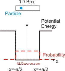
The higher order terms follow the same pattern.

When using a thermodynamic model, one first determines the thermal average of the dipole moment in the presence of an electric field (see below). Quantum models require the expectation value of the dipole operator (see the tutorial on the quantum calculation of the polarizability). Then, the polarizability and higher order terms are determined through differentiation.

A Thermodynamic Model

As an example of the above approach, we consider a particle in a one-dimensional box, as shown below.

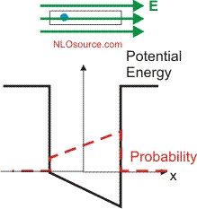
The thermodynamic probability density of finding the particle at any point in the well is the same, while the probability density outside the well is zero, as shown by the dashed line.

In the presence of a uniform and static electric field, the well tips, as shown below.

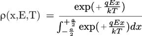
The probability density of finding the charged particle is larger to the right due to the electric field bias. As a function of temperature, T, applied electric field, E, and particle's charge q, the probability density is given by,

.

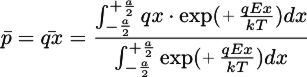
The expectation of the dipole operator is given by

,

which yields

.

Note that in the limit of infinite temperature, the polarizability vanishes, as expected on the grounds of the physical argument that when the electric field is negligible, the charge is on average at the origin.

Exercises

1. Verify the above result for the polarizability of a particle in a 1D box and calculate the hyperpolarizability.
2. Calculate the second hyperpolarizability of the particle in a 1D box, which is defined by

3. Calculate μ₀ (the static dipole moment), α, β, and γ for a freely rotating rigid molecule with permanent dipole moment μ if it is in thermal equilibrium with a bath of temperature T.
4. For the dynamic nonlinear spring as described in Chapter 1 of Boyd's book on Nonlinear Optics, create a surface plot β(ω₁,ω₂) that clearly shows all of the resonance's.